Details about river forcing files

Details about river forcing files#

We use the dataretrieval-python package to access USGS NWIS river data.

Background information#

There is a report from the Coast Survey Development Laboratory modeling group’s development of the CIOFS model, and this along with two nowcast rivers forcing files we received from the NOAA OFS modeling group is what we used to create our own river forcing files, trying to follow the same logic when possible.

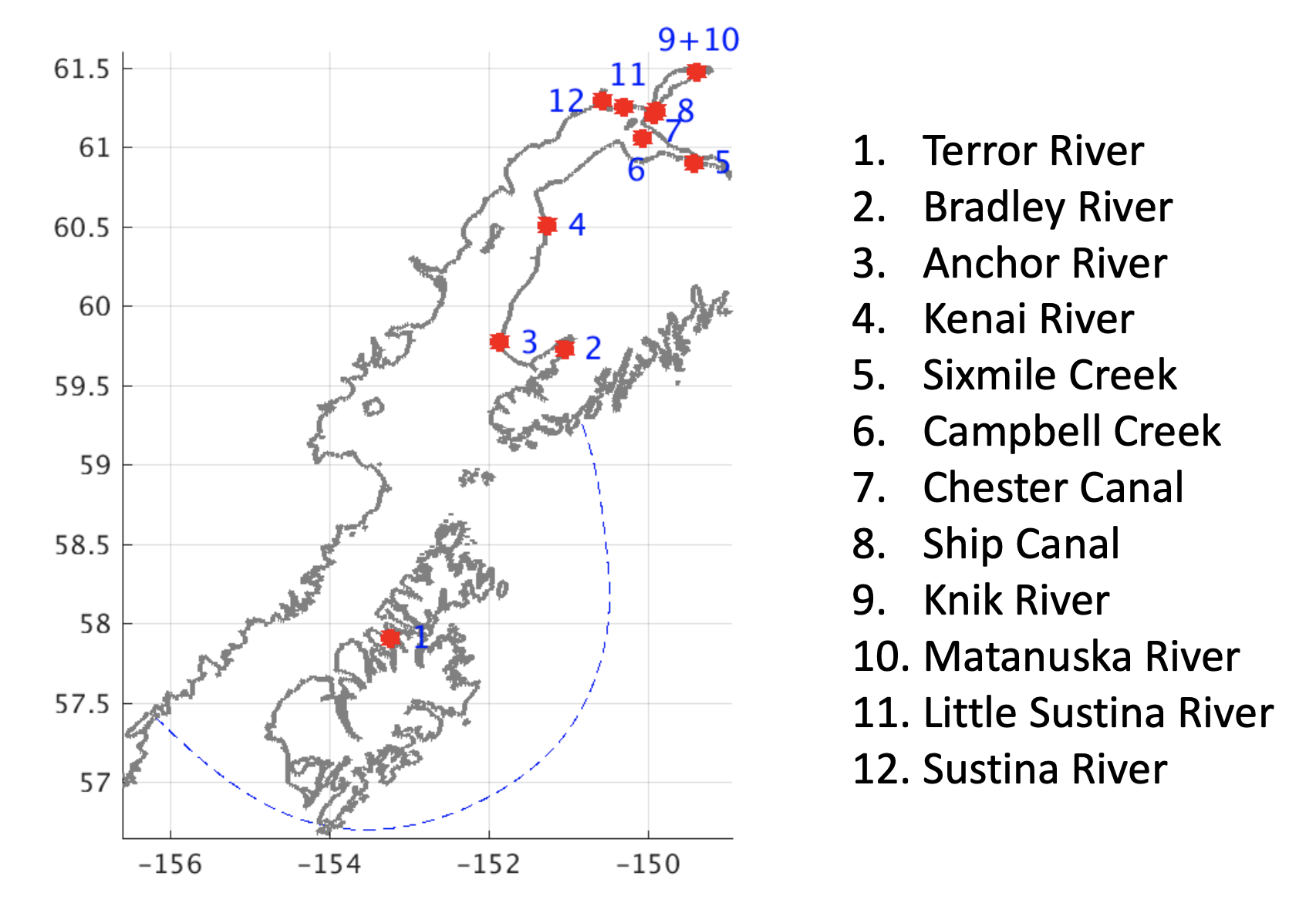
Freshwater is included in the CIOFS model as 12 rivers spread over 36 river points. The rivers included are listed in the left column here:

Number	River Station in Model	USGS Station Used: Discharge	USGS Station Used: Water temp	Notes
1	15295700: Terror River at mouth near Kodiak, AK	15295700	15295700
2	15239070: Bradley River near Tidewater near Homer, AK	15239070	15239070
3	15239900: Anchor River near Anchor Point, AK	15239900	15239900
4	15266300: Kenai River at Soldotna, AK	15266300	15266300
5	15271000: Sixmile Creek near Hope, AK	15271000	15258000: Kenai River at Cooper Landing AK
6	15274600: Campbell Creek near Spendard, AK	15274600	15276000: Ship Canal near Anchorage AK
7	15275100: Chester Canal at Arctic Boulevard at Anchorage, AK	15275100	15276000: Ship Canal near Anchorage AK
8	15276000: Ship Canal near Anchorage, AK	15276000	15276000
9	15281000: Knik River near Palmer, AK	15281000	15284000: Matanuska River near Palmer, AK
10	15284000: Matanuska River near Palmer, AK	15284000	15284000
11	15290000: Little Susitna River near Palmer, AK	15290000	15290000
12	15292780: Susitna River at Sunshine, AK	15292000: Susitna River at Gold Creek AK	15292780	Discharge from 15292000 is multiplied by 2.

We followed what we saw in two river forcing files from the CIOFS group, and ascertained some details to include in the data processing:

River salinity is set to 0.005 for all rivers
River temperature is never allowed below 1 degree Celsius.
Use all data in UTC.

River input locations are shown on this map from the development report:

../_images/afc25755711a0899bb8872252b6c003a6a829f4dd72df6300620340fee507791.png

General approach#

This is a text flow chart of the logic in create_river_roms.py. Logic flows first down, then across a line and stops if “Done”, otherwise continues down the list. No gage data is used in this analysis.

Discharge#

get discharge data.
Check for:
1. empty → Use mean time series
2. fully present (all time stamps for date range) with good data flags (“A” or “P” flag) → use, done.
3. Reindex to fill all missing times with nans
4. Deal with other flags (ice or equipment malfunction): fill all with nan (“A, e” or “P, e” flags are ok)
5. Check gap lengths.
Has gaps in data. Process all gaps. If gaps are:
1. Less than 7 days → interpolate
2. Over 7 days → Use mean time series.

Water temperature#

get temp data.
Check for:
1. empty → use mean data. Done.
2. fully present (all time stamps for date range) with good data flags (“A” or “P” flag) → use, done.
3. Reindex to fill all missing times with nans
4. Check gap lengths.
Has gaps in data. Process all gaps. If gaps are:
1. Less than 8 days → interpolate
2. Over 8 days → use mean data

More details#

Station substitutes are listed in the Station Table above. There is one station substitute for discharge, and more for water temperature.
The model development report stated that because the desired Station 15292780 is not available for a long time, they substituted discharge from Station 15292000 and multiplied by 2 to approximate the difference seen between the two stations.
The model development report stated that temperatures from Bradley River (Station 15292780) were used for all stations. We decided to allow the water temperature to vary in space.
We use mean time series for water temperature and discharge when real-time data is not available.

Details for each point are below.

Discharge for Station 15292780#

The NOAA Report states that they used Station 15292000 discharge multiplied by 2 to replace discharge from Station 15292780 since Station 15292780 has a relatively short lifespan. We do the same in our simulations. Here is the comparison of the daily means for these two time series, including the multiplication factor. The match is reasonable.

../_images/85f3cfc5650c0a1b4988f84f302c138926711400b49e4813449fa40d48dcff2d.png

Geographic variation of water temperature#

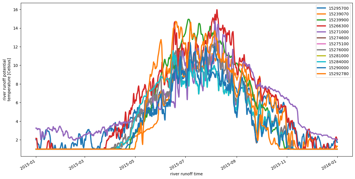
The development report states that Bradley River (15239070) was used to represent all rivers in the model. We chose to allow for spatially-varying data. This one year of data shows an example of the variation in temperature data across the region. There is a fair amount of variation, but we have run no tests to analyze how impactful the variation is for the final results.

../_images/10a5522efa75ba9a19de9691be6913eb47c0286883de91f2200cec09b6b0d0b2.png

Mean time series#

../_images/92b0ef0b423d468756b2c350b0e5df80cbac2e9626911860bef7fde015645ec8.png

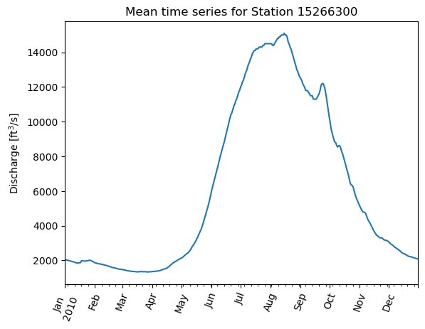
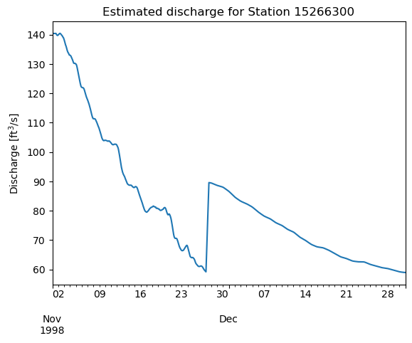
The impact of substituting the mean time series data in for the discharge when needed is that there could be a jump between the two signals. We simply perform a 12 hour rolling mean on the discharge signal at the end of processing in order to improve this, but it is a small measure; there will still be some unrealistic jumps in the river signals. However, we think it is worth it to have more freshwater entering the model domain when we know it is present and important to the region.

../_images/3c45589ba103772fe3b9789a5f39e275a741ead1a56bb5b0c2d996796c2fdeba.png

Comparing Axiom and NOAA versions of two river forcing files#

We received two example nowcast river forcing files which we recreate here as a comparison with our methods. Note that in order to compare with the four-day nowcast files we do two things differently from our month-long hindcast forcing files:

interpolate under 2 days and use gage or mean time series data over 2 days instead of 8 days for both
do not apply a rolling mean of 12 hours

The main differences seen below are:

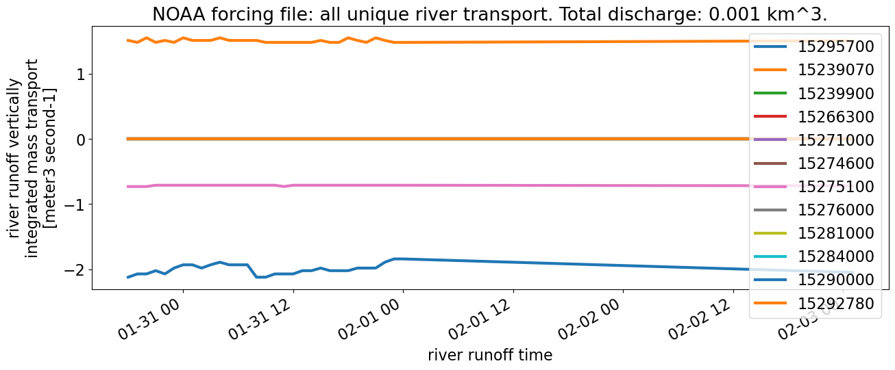
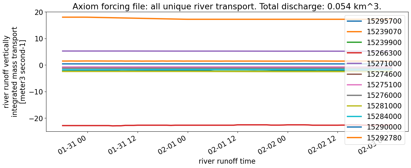
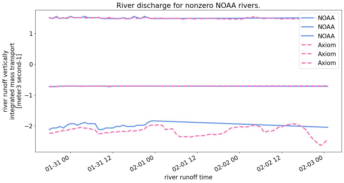
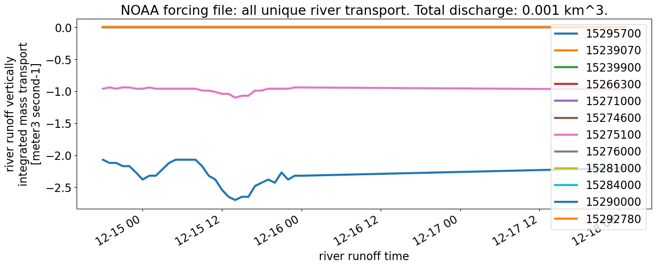
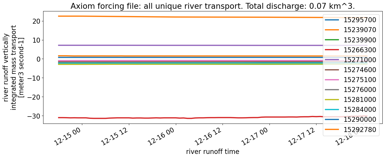
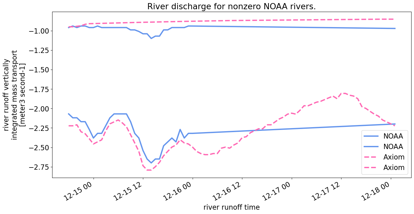
We do not estimate discharge from gage data, but we do include discharge from the statistical mean time series for the station if there are any iced or equipment malfunction flags. Because of this, we include much more freshwater input as compared with the example files. NOAA’s file does include an estimate of discharge from gage data from one river, but not from other rivers.
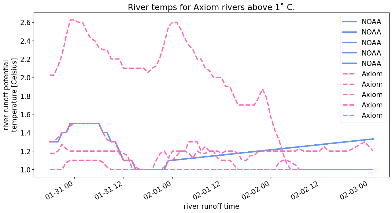
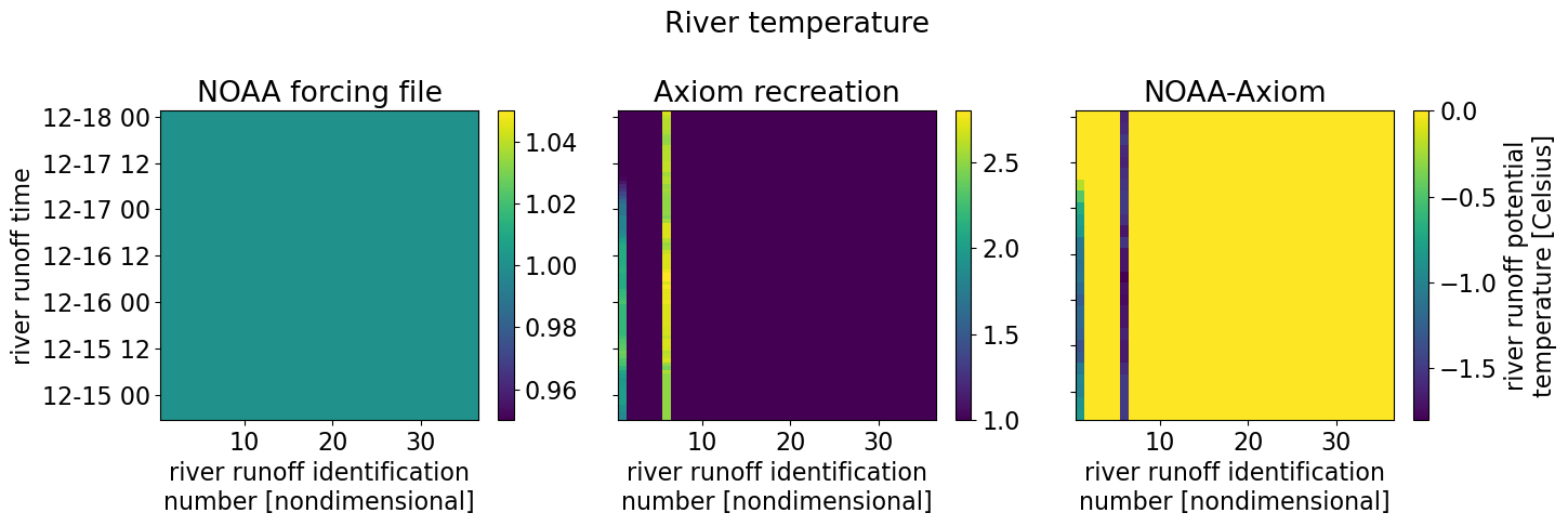
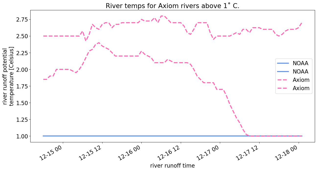
We used geographically-varying water temperature data, whereas the NOAA groups use data only from Bradley River (Station 15239070). When real-time water temperature data is not available, we use the statistical mean time series for the station. When a station has never had an instrument to measure water data, we have a replacement station as shown in the station table.
The nowcast forcing files are created by NOAA at the mid point of the time series such that they use the real-time data up until the start of the simulation, and the second half of the forcing is a simple linear extrapolation of the available data (which is why they appear as straight lines for those times).

Show code cell content Hide code cell content

def plot_comparison(ds, dscompare):
    
    plt.rc('font', size=16)
    
    color_noaa = "cornflowerblue"
    color_axiom = "hotpink"
    kwargs_line = {"x": "river_time", "lw": 3}
    kwargs_noaa = {"color": color_noaa, "label": "NOAA"}
    kwargs_axiom = {"color": color_axiom, "label": "Axiom", "ls": "--"}
    
    fig, axes = plt.subplots(1, 3, figsize=(15,5))
    ds["river_transport"].plot(ax=axes[0], cbar_kwargs={"label": ""})
    dscompare["river_transport"].plot(ax=axes[1], cbar_kwargs={"label": ""})
    (ds["river_transport"] - dscompare["river_transport"]).plot(ax=axes[2])
    axes[0].set_title("NOAA forcing file")
    axes[1].set_title("Axiom recreation")
    axes[1].set_ylabel("")
    axes[1].set_yticklabels("")
    axes[2].set_title("NOAA-Axiom")
    axes[2].set_ylabel("")
    axes[2].set_yticklabels("")
    fig.suptitle("River discharge")
    plt.tight_layout()

    noaa_discharge = round(float(abs(ds['river_transport']).sum()*3600/1000**3), 3)  # m^3/s * 3600 s for hour * (1km/1000m)^3
    axiom_discharge = round(float(abs(dscompare['river_transport']).sum()*3600/1000**3), 3)  # m^3/s * 3600 s for hour

    unique_inds = list(set([station_list_file.index(station_list_file[i]) for i in range(nrivers)]))
    labels = [station_list_file[i] for i in unique_inds]
    ds["river_transport"].isel(river=unique_inds).plot.line(**kwargs_line, figsize=(15,5));
    plt.title(f"NOAA forcing file: all unique river transport. Total discharge: {noaa_discharge} km^3.")
    plt.legend(labels)
    dscompare["river_transport"].isel(river=unique_inds).plot.line(**kwargs_line, figsize=(15,5));
    plt.title(f"Axiom forcing file: all unique river transport. Total discharge: {axiom_discharge} km^3.")
    plt.legend(labels)

    # pull over rivers that have nonzero transport from original file
    ibool = abs(ds["river_transport"].sum(dim="river_time")) > 0
    ind = ds["river"][ibool] - 1
    key = "river_transport"
    ds[key].isel(river=ind).plot.line(**kwargs_line, **kwargs_noaa, figsize=(15,7));
    dscompare[key].isel(river=ind).plot.line(**kwargs_line, **kwargs_axiom);
    plt.legend()
    plt.title("River discharge for nonzero NOAA rivers.")

    fig, axes = plt.subplots(1, 3, figsize=(15,5))
    ds["river_temp"].isel(s_rho=0).plot(ax=axes[0], cbar_kwargs={"label": ""})
    dscompare["river_temp"].isel(s_rho=0).plot(ax=axes[1], cbar_kwargs={"label": ""})
    (ds["river_temp"] - dscompare["river_temp"]).isel(s_rho=0).plot(ax=axes[2])
    axes[0].set_title("NOAA forcing file")
    axes[1].set_title("Axiom recreation")
    axes[1].set_ylabel("")
    axes[1].set_yticklabels("")
    axes[2].set_title("NOAA-Axiom")
    axes[2].set_ylabel("")
    axes[2].set_yticklabels("")
    fig.suptitle("River temperature")
    plt.tight_layout()

    # pull over rivers that have non-one temp from Axiom file
    ibool = (dscompare["river_temp"].isel(s_rho=0) > 1).any(dim="river_time")
    ind = dscompare["river"][ibool] - 1

    key = "river_temp"
    ds[key].isel(s_rho=0, river=ind).plot.line(**kwargs_line, **kwargs_noaa, figsize=(15,7));
    dscompare[key].isel(s_rho=0, river=ind).plot.line(**kwargs_line, **kwargs_axiom);
    plt.legend()
    plt.title("River temps for Axiom rivers above 1˚ C.")
        

December 2022 file#

The total amount of discharge input over the 4 days in the forcing file is much larger from the Axiom file: 0.07 km\(^3\) compared with 0.001 km\(^3\) from the NOAA file. However, for the two rivers that do have discharge from the NOAA file (most are all 0s), we are able to estimate a good match (“River discharge for nonzero NOAA rivers”).

River temperature data is all 1s in the NOAA file but we allow for spatial variation and see in the comparison (“River temps for Axiom rivers above 1 C”) this variation. Note than any temperatures below 1 degree are set to 1 degree.

../_images/d489a35df155a0f691fa17836dd0415cc72fccaa9a3cf265e8692921f3a6715c.png

../_images/4ad7d1192883fe98013341f1dc8f95cfe78460666e261121adc6850311d7ce67.png

../_images/decc54168ea6ec5f7ff807d0e85be6c20699b32f4b1039fdd1c4e36183be4256.png

../_images/d18cbb0f81c1a89b3828773ae8e8cb70b886a0536ef11b91298147c6ab8e1faf.png

../_images/3b4a7e1730cc145a7c80dad780a97cc62a02bfa3d20c2e20ed382544e7d447fc.png

../_images/6985c7ce832fae36e13eab908583625ec657d3777b6bc0210986bfbddd5acc0e.png

January 2023 file#

For the same reasons previously listed, the discharge is much higher from the Axiom file: 0.06 km\(^3\) compared with 0.001 km\(^3\) from the NOAA file. For the rivers that we estimate in the same way as NOAA, we get similar results.